Residual Lives, Hazard Rates, and Long Tails (Part I)

This is the third series of posts I’m writing on topics related to what we are covering in our book on heavy-tails (which I discussed in an earlier post). The first two were on the catastrohphe principle (subexponential distributions) and power laws (regularly varying distributions). This time I’ll focus on connections between residual life, hazard rate, and long tailed distributions.

Residual life in our daily lives

Over the course of our days we spend a lot of our time waiting for things — we wait for a table at restaurants, we wait for a subway train to show up, we wait for people to respond to our emails, etc. In such scenarios, we hold on to the belief that, as we wait, the likely amount of remaining time we will need to wait is getting smaller. For example, we believe that, if we have waited ten minutes for a table at a restaurant, the expected time we have left to wait should be smaller than it was when we arrived and that, if we have waited five minutes for the subway, then our expected remaining wait time should be less than it was when we arrived.

In many cases this belief holds true. For example, as other diners finish eating, our expected waiting time for a table at a restaurant drops. Similarly, subway trains follow a schedule with (nearly) deterministic gaps between trains and thus, as long as the train is on schedule, our expected remaining waiting time decreases as we wait. However, a startling aspect of heavy-tailed distributions is that this is not always true. For example, if you have waited a very long time past the scheduled arrival time for a subway train, then it is very likely that there was some failure and the train may take an extremely long time to arrive, and so your expected remaining waiting time has actually increased while you waited. Similarly, if you are waiting for a response to an email and have not heard for a few days, it is likely to be a very long time until a response comes (if it ever does).

The above examples highlight another fundamental distinction between light-tailed distributions (e.g. restaurant waiting times) and heavy-tailed distributions (e.g. email waiting times). To make the contrast even more clear, we can illustrate the same distinction using our classic examples of heavy-tailed and light-tailed distributions: incomes and heights. If we know someone is taller than 6′, then it is most likely that they are only a few inches taller; but if we know someone has more than $1 million, then it much more likely that they are multi-millionaires than that they are just barely millionaires.

All these examples highlight that, as with scale-invariance and the catastrophe principle, the behavior we expect to see is aligned with what happens under light-tailed distributions and so, upon first encounter, the behavior of heavy-tailed distributions is mysterious. Said in a slightly more formal manner, we expect that if we have waited a long time the remaining waiting time, i.e., the residual life, should have decreased, and so it is particularly jarring that under heavy-tailed distributions the residual life will have increased dramatically.

In this series of posts we explore the residual life of heavy-tailed distributions in order to build intuition for the counterintuitive phenomena described above. To do this, we start by exploring the distribution of residual life via two common measures: the hazard rate function and the mean residual life function. We then study the relationship between heavy-tailed distributions and properties of the hazard rate and the mean residual life, which leads us to the formalization of a subclass of heavy-tailed distributions, termed long-tailed distributions, that we explore in depth.

Residual lives and hazard rates

The residual life of a distribution refers to the remaining waiting time given that you have already been waiting for some amount of time. Thus, it crucially depends on how long you have waited already; and so it is clear that it is a conditional concept. Formally, we define the residual life distribution as follows.

Definition 1 For a nonnegative random variable ${X}$ with distribution function ${F,}$ the residual life distribution ${R_x(t)}$ is defined such that

$\displaystyle \bar{R}_x(t) = 1-R_x(t) = \mathop{\mathbb P}\{X>x+t|X>x\} = \frac{\bar{F}(x+t)}{\bar{F}(x)}.$

Thus, ${R_x(t)}$ is the distribution of the waiting time given that you have already waited for ${x}$ time. Though it is a relatively simple concept, the residual life is compelling because of the wide variety of applications it has found, ranging from the insurance assessment and reliability theory to the social sciences, where it has found use in studying the lifetimes of everything from the length of wars to human life expectancies.

To begin to get a feel for the residual life distribution, let us consider some examples. Conveniently, it tends to be quite straightforward to calculate ${\bar{R}_x(t)}$ for common distributions. For example, ${\bar{R}_x(t)}$ for the Pareto distribution can be computed as follows

$\displaystyle \text{Pareto: } \bar{R}_x(t) = \frac{\left(\frac{x+t}{x_m}\right)^{-\alpha}}{\left(\frac{x}{x_m}\right)^{-\alpha}} = \left(1 + \frac{t}{x}\right)^{-\alpha}$

Interestingly, this highlights that, for any ${x}$ , ${\bar{R}_x(t)}$ follows a Burr distribution, and thus has a regularly varying tail.

Similarly, the residual life distribution of the Exponential can be calculated easily.

$\displaystyle \text{Exponential: } \bar{R}_x(t) = \frac{e^{-\mu(x+t)}}{e^{-\mu x}} = e^{-\mu t}$

A striking aspect of the above is that ${\bar{R}_x(t)=\bar{F}(t)}$ . This is a restatement of the “memoryless” property of the exponential distribution, which says that regardless of how long you have waited so far, the distribution of the remaining time you have to wait is exactly the same as if you just arrived. This is a particularly special property of Exponential distributions, which are the only continuous distributions that are memoryless.

Finally, let us consider the the residual life of the Weibull distribution. Again, it is simple to calculate.

$\displaystyle \text{Weibull: } \bar{R}_x(t) = \frac{e^{-\mu(x+t)^k}}{e^{-\mu x^k}} = e^{-\mu (x+t)^k+\mu x^k}$

However, though it is simple to calculate ${\bar{R}_x(t)}$ for the Weibull, the resulting form is not particularly informative without a deeper study.

More generally, despite the fact that the residual life distribution is typically easy to derive, it it often useful (or even necessary) to look at statistics of the residual life distribution in order to obtain insight into its behavior. There are two statistics that are most commonly used: the mean residual life and the hazard rate.

The mean residual life

Of course whenever we consider a distribution, it is natural to use its mean in order to obtain insight. In this case, because residual life is a conditional concept that depends on the how long you have waited so far, the mean of the residual life distribution is actually a function. In particular, the mean residual life function is defined as follows.

Definition 2 For a nonnegative random variable ${X}$ with distribution function ${F,}$ define the mean residual life (MRL) function ${m(x) = \mathop{\mathbb E}[X-x\ |\ X>x].}$ Equivalently

$\displaystyle m(x) = \int_0^{\infty} \bar{R}_x(t) dt = \int_0^\infty \frac{\bar{F}(x+t)}{\bar{F}(x)} dt \ \ \ \ \ (1)$

Though the definition of the mean residual life function ${m(x)}$ is far less common that of the density function ${f(x)}$ , the distribution function ${F(x)}$ , or moment generating function ${M(s)}$ , like these ${m(x)}$ completely determines the distribution when the distribution has a finite mean. Thus, for example, it is possible to “invert” ${m(x)}$ to calculate the distribution function ${F(x)}$ .

The simplicity of the definition of the mean residual life means that it is typically not hard to compute ${m(x)}$ for common distributions. To illustrate the behavior of ${m(x)}$ let us return to the examples of the Pareto, Exponential, and Weibull. For the Pareto distribution, it is quite straightforward to calculate ${m(x)}$ . In particular, assuming that the mean is finite ( ${\alpha>1}$ ), we have

$\displaystyle \text{Pareto: } m(x) = \int_0^\infty \bar{R}_x(t) dt = \int_0^\infty \left(1+\frac{t}{x}\right)^{-\alpha} dt = \frac{x}{\alpha-1}.$

Interestingly, from the above we see that the mean residual life of the Pareto distribution is increasing, and grows unboundedly with ${x}$ . In particular, under a Pareto distribution, the expected remaining waiting time grows linearly with the amount of time you have waited so far.

The calculation of the mean residual life is also straightforward for the Exponential distribution

$\displaystyle \text{Exponential: } m(x) = \int_0^\infty \bar{R}_x(t) dt = \frac{1}{\mu} \int_0^\infty \mu e^{-\mu t} dt = \frac{1}{\mu}$

This derivation highlights a consequence of the memoryless property of Exponential distributions — the mean residual life is constant with respect to ${x}$ , specifically ${m(x)=1/\mu=\mathop{\mathbb E}[X]}$ . That is, the expected remaining waiting time is the same as when you first arrived, regardless of how long you have waited.

Though it has been straightforward to calculate the residual life function ${m(x)}$ for the Pareto and the Exponential, it is not always easy. The example of the Weibull distribution highlights this fact. In particular, it is difficult to derive an explicit formula for ${m(x)}$ for the Weibull distribution.

The hazard rate

A second important statistic of the residual life distribution is the hazard rate. We have already mentioned the hazard rate a few times in the book, but here we will introduce it more formally and study it in detail, since it is fundamentally related to the residual life distribution. In particular, the residual life distribution ${\bar{R}_x(t)}$ looks at the remaining waiting time given that you have already waited for a certain amount of time ${x}$ , and the hazard rate can be thought of as the likelihood of the wait time ending now, given that you have waited ${x}$ time already. Thus, as we will see, the hazard rate is tied to the density of the residual life distribution.

Formally, the hazard rate is defined as follows.

Definition 3 For a nonnegative random variable ${X}$ with distribution function ${F}$ and density function ${f}$ , define the hazard rate, a.k.a., the failure rate, as ${q(x) = \frac{f(x)}{\bar{F}(x)}.}$ Further, define the cumulative hazard as ${Q(y) = \int_0^y q(x) dx}$ .

It is easy to see that the hazard rate and the residual life are intimately related. In particular, the hazard rate corresponds to the density of the residual life distribution evaluated at zero.

$\displaystyle \bar{R}'_x(0) = \frac{d}{dt}\left(\frac{\bar{F}(x+t)}{\bar{F}(x)} \right)|_{t=0} = \frac{-f(x+t)}{\bar{F}(x)}|_{t=0} = \frac{-f(x)}{\bar{F}(x)}=-q(x)$

Further, the hazard rate is intrinsically tied to the tail of the distribution. To see this, note that

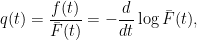
$\displaystyle q(t) = \frac{f(t)}{\bar{F}(t)} = -\frac{d}{dt} \log \bar{F}(t),$

and so

$\displaystyle Q(x) = -\log \bar{F}(x),$

which gives

$\displaystyle \bar{F}(x) = e^{-Q(x)} = e^{-\int_0^x q(t) dt}.$

As a consequence of the above, it is easy to see that the hazard rate and the mean residual life are also closely related. In particular, as long as both exist, we have

$\displaystyle m(x) =\int_0^{\infty} e^{-\int_{x}^{x+t} q(y)dy } dt, \ \ \ \ \ (2)$

which highlights that if the hazard rate is monotonically decreasing (increasing) then the mean residual life will be monotonically increasing (decreasing). Further, it is possible to show that

$\displaystyle m'(x) = m(x)q(x)-1. \ \ \ \ \ (3)$

The first of these is easy to verify, but the second requires some effort.

To get a feeling for the behavior of the hazard rate let us return again to our examples of the Pareto, Exponential, and Weibull. Either computing directly, or using the above relationships it is straightforward to see that the hazard rates of the Pareto and the Exponential are as follows.

$\displaystyle \text{Pareto: } q(t) = \frac{\alpha}{t}$

$\displaystyle \text{Exponential: } q(t) = \mu.$

Thus, the Pareto has a hazard rate that decreases to zero, while the Exponential has a constant hazard rate. This contrast is interesting: the memoryless property of the Exponential distribution means that the likelihood that your waiting time ends is unchanging as you wait, while under the Pareto distribution the likelihood that your waiting time ends decreases to zero as you wait.

It is also straightforward to compute the hazard rate of the Weibull distribution, which is in contrast to the difficulty of computing ${m(x)}$ in this case. In particular, the hazard rate of the Weibull satisfies the following

$\displaystyle \text{Weibull: } q(t) = \frac{k}{\lambda}\left(\frac{t}{\lambda}\right)^{k-1}$

The form of the hazard rate under the Weibull distribution highlights a similar contrast to what we saw between the Pareto and the Exponential, only more extreme. When ${k>1}$ the hazard rate is increasing (and thus the mean residual life is decreasing), which means that the likelihood your wait ends increases as you wait, while when ${k<1}$ the hazard rate is decreasing (and thus the mean residual life is increasing), similarly to that of the Pareto distribution. Of course, ${k=1}$ corresponds to the case of the Exponential distribution, and so the hazard rate is constant.

Heavy tails and residual lives

The simple examples of the Pareto, Exponential, and Weibull that we have used so far highlight exactly the contrast between light-tailed and heavy-tailed distributions that we have discussed informally in the introduction to this post: if we have waited a long time, then under light-tailed Weibull distributions the expected remaining waiting time will have decreased, while under the heavy-tailed Weibull and Pareto distributions the expected remaining waiting time will have increased dramatically.

In particular, we have seen that under the light-tailed Weibull the mean residual life is decreasing and the hazard rate is increasing, while under the heavy-tailed Weibull and Pareto distributions the mean residual life is increasing unboundedly and the hazard rate is decreasing to zero. The fact that these three distributions all have monotonic hazard rates and mean residual lives points us toward the importance of this property, and in particular, motivates the definition of the following four classes of distributions.

Definition 4 A nonnegative distribution ${F}$ with mean residual life function ${m}$ is said to have increasing/decreasing mean residual life (IMRL/DMRL) if ${m(x)}$ is increasing/decreasing in ${x}$ for all ${x}$ such that ${F(x)\in(0,1)}$ .

Definition 5 A nonnegative distribution ${F}$ with hazard rate ${q}$ is said to have increasing/decreasing hazard rate (IHR/DHR) if ${q(t)}$ is increasing/decreasing in ${t}$ for all ${t}$ such that ${F(x)\in(0,1)}$ .

Clearly, heavy-tailed Weibull and Pareto distributions are IMRL and DHR; while light-tailed Weibull distributions are DMRL and IHR. Given these examples and the relationship between the hazard rate and the mean residual life, one would expect a strong connection between the DMRL/IMRL and IHR/DHR, and this is indeed the case. In fact, it follows immediately from (2) that the IHR class is contained within the DMRL class and the DHR class is contained within the IMRL class.

Theorem 6 All distributions with an increasing (decreasing) hazard rate have a decreasing (increasing) mean residual life, i.e., IHR ${\subseteq}$ DMRL and DHR ${\subseteq}$ IMRL.

At this point it is natural to notice that, because the Exponential distribution has constant mean residual life and hazard rate, it is, in some sense, the boundary between the IHR and DHR classes and between the IMRL and DMRL class. Of course, Exponential distributions also serve as the boundary between light-tailed and heavy-tailed distributions, and so it is quite tempting to think of IMRL/DHR distributions has “heavy-tailed” and DMRL/IHR distributions as “light-tailed”. In fact, the temptation is so strong that in some disciplines, IMRL is used as a defining property of “heavy-tailed” distributions. However, one must be careful with this view since “heavy-tailed” and IMRL/DHR are actually quite different concepts, as are “light-tailed” and DMRL/IHR.

In particular, it is easy to construct examples of IMRL and DHR distributions that are not heavy-tailed and examples of heavy-tailed distributions that are not IMRL or DHR. For example, a heavy-tailed distribution that is not IMRL or DHR is the Burr distribution. Though the ${m(x)}$ is eventually increasing and ${q(x)}$ is eventually decreasing for the Burr distribution, they are monotonic over the entire distribution.

Similarly, it is easy to construct examples of light-tailed distributions that are IMRL and IHR. In particular, the Hyperexponential distribution is an example of a light-tailed distribution that has increasing mean residual life and a decreasing hazard rate. Recall that the Hyperexponential distribution is a mixture of exponential distributions where with probability ${p_i}$ a sample is drawn from an Exponential distribution with rate ${\mu_i}$ , for ${i=1,\ldots,n}$ with ${\sum p_i = 1}$ .

Correspondingly, one must be careful to distinguish “light-tailed” from DMRL. Here, it is true that all DMRL and IHR distributions are light-tailed. However, there are many examples of light-tailed distributions that are not DMRL or IHR. An easy example to highlight this is a bounded Pareto distribution, i.e., a distribution that has a Pareto body, but has a finite upper bound. For such a distribution, ${m(x)}$ is initially increasing, since the unbounded Parteo is IMRL and DHR, but eventually decreases to zero, since there is an upper bound on the size.

Long-tailed distributions

The previous discussion has highlighted that one must be careful in connecting “heavy-tailed” with the concepts of “increasing mean residual life” and “decreasing hazard rate”. In particular, there are many examples of light-tailed distributions that are IMRL and DHR. However, if we think again about the informal examples that we discussed at the beginning of the post, it becomes clear that IMRL and DHR are too “precise” to capture the phenomena we were describing. For example, if we return to the case of waiting for a response to an email. It is not that we expect our remaining waiting time to be monotonically increasing as we wait. If fact, we are very likely to get a response quickly, and so the expected waiting time should drop initially (and the hazard rate should increase initially). It is only after we have waited a “long” time already, in this case a few days, that we expect to see a dramatic increase in our residual life. Further, in the extreme, if we have not received a response in a month, we can reasonably expect that we may never receive a response, and so the mean residual life is, in some sense, growing unboundedly, or equivalently the hazard rate is decreasing to zero. The example of waiting for a subway train highlights the same issues. Initially, we expect that the mean residual life should decrease, because if the train is on schedule, things are very predictable. However, once we have waited a long time beyond when the train was supposed to arrive, it likely means something went wrong, and could mean the train has had some sort of mechanical problem and will never arrive.

These examples highlight two important aspects that need to be captured in a formalization of this phenomena. First, they highlight that strict monotonicity of the residual life is not crucial (or desirable), and that we should instead focus on the behavior of the tail. And, second, they highlight that the phenomena we would like to capture includes the fact that the residual life distribution “blows up”, in the sense that if we have waited a very long time we should expect to wait forever. Note that this property is true of heavy-tailed Weibull and Pareto distributions, but is not true of the light-tailed distributions that are a part of the IMRL and DHR classes. For example, the Hyperexponential distribution with rate parameters ${\mu_1,\ldots,\mu_n}$ has a mean residual life that is upper bounded by ${\max_i(1/\mu_i)}$ .

These two observations lead us to the definition of the class of long-tailed distributions, which is where we will start the next post.

4 thoughts on “Residual Lives, Hazard Rates, and Long Tails (Part I)”

Pingback: Rigor + Relevance | Residual Lives, Hazard Rates, and Long Tails (Part II)
Roy Smith
July 30, 2015
8:52 am

Hi Adam,

Great blog series.

I suspect that there is a typo in the following statement about the hazard rate of the Weibull distribution:

“When {k>1} the hazard rate is increasing (and thus the mean residual life is increasing),”

Shouldn’t it be “mean residual life is decreasing”?

Cheers, Roy

- Adam Wierman
  July 30, 2015
  10:17 am
  
  Thanks for the comment and the catch — I’ve fixed the typo!
  
hasan
January 24, 2024
7:21 pm

Thank you for nice introduction to the concepts of hazard function and mean residual time. I want to ask whether there is a classification of distribution such that hazard function is less than or equal to the reciprocal of mean residual time, i.e. 1/m(t) >= h(t) for all t.