Solution to puzzle: produce or learn?

This post is a solution to the puzzle in the last post.

The optimal strategy has a very simple form: there is a time 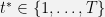such that ( denotes optimal quantities)

• only learn () before time ;
• only produce () from time  on.

Another puzzle: produce or learn?

When our kids were small, they were in sports teams (basketballs, baseball, soccer, …).  Their teams would focus on drills early in the season, and tournaments late in the season.  In violin, one studies techniques (scales, etudes, theory, etc.) as well as musicality (interpretation, performance, etc).   In (engineering) research, we spend a lot of time learning the fundamentals (coursework, mathematical tools, analysis/systems/experimental skills, etc.) as well as solving problems in specific applications (research). What is the optimal allocation of one’s effort in these two kinds of activities?

This is a complex and domain-dependent problem.  I suppose there is a lot of serious empirical and modeling research done in social sciences (I’d appreciate pointers if you know any).  But let’s formulate a ridiculously simple model to make a fun puzzle.

1. Consider a finite horizon t = 1, 2, …, T.   The time period t can be a day or a year.  The horizon T can be a project duration or a career.
2. Suppose there are only two kinds of activities, and let’s call them production and learning.  Our task is to decide for each t, the amount of effort we devote to produce and to learn.  Call these amounts p(t) and l(t) respectively.
3. These activities build two kinds of capabilities.  The fundamental capability L(t) at time t depends on the amount of learning we have done up to time t-1, L(t) := L(l(s), s=1, …, t-1).  The production capability P(t) at time t depends on the amount of effort we have devoted to production up to time t-1, P(t) := P(p(s), s=1, …, t-1).   We assume the functions L(l(s), s=1, …, t-1) and P(p(s), s=1, …, t-1) are increasing and time invariant (i.e., they depend only on the amount of effort already devoted, but not on time t).
4. The value/output we create in each period t is proportional to the time p(t) we spend on production multiplied by our overall capability at time t.   Our overall capability is a weighted sum P(t) + mL(t) of fundamental and production capabilities, with m>1.

Goal: choose nonnegative (p(t), l(t), t=1, …, T) so as to maximize the total value subject to for all t=1, …, T.

The assumption m>1 means that the fundamentals (quality) are more important than mere quantity of production.  The constraint says that in each period t, we only have a finite amount of energy (assume a total of 1 unit) that can be devoted to produce and learn.  On the one hand, we want to choose a large p(t) because it not only produces value, but also increases future production capabilities P(s), s=t+1, …, T.  On the other hand, since m>1, choosing a large l(t) increases our overall capability more rapidly, enhancing value.  What is the optimal tradeoff?

We pause to comment on our assumptions, some of which can be addressed without complicating our model too much.

Caveats.  On the outset, our model assumes every activity can be cleanly classified as building either the fundamental capability or the production capability.  In reality, many activities contribute to both.  Moreover, the interaction between these two activities is completely ignored, except that they sum to no more than 1 unit.  For example, production (games, performance, research and publication, etc) often provides important incentives and contexts for learning and influences strongly the effectiveness of learning, but our function L is independent of  p(s).  The time invariance assumption in 3 above implies that we retain our capabilities forever after they are built; in reality, we may lose some of them if we don’t continue to practice.  If we think of P(t)+mL(t) as a measure of quality, then our objective function assumes that there is always positive value in production, regardless of its quality.  In reality, production of poor quality may incur negative value, even fatal.

 A puzzle

A simple puzzle is the special case where the capabilities depend on (are) the total amounts of effort devoted, i.e.,

Despite its nonconvexity, the problem can be explicitly solved and the optimal strategy turns out to have a very simple structure.  I will explain the solution in the next post and discuss whether it agrees, to first order, with our intuition and how some of the disagreements can be traced back to our simplifying assumptions.

A holiday puzzle: solution

I now discuss two solutions to the puzzle described in the last post — one for the special case of a linear grid, and the other for the general 2D grid.  I thank Johan Ugander and Shiva Navabi for very useful pointers (see the Comment in the last post, and a funny nerd snipe comic) — I will return to them below.  But first, here is a simple heuristic solution.

A holiday puzzle

I am afraid of gifts, both receiving and giving.  Luckily, I have been largely spared having to confront this challenge.  I am often (rightly) criticized that in rare occasions when I give, the gifts are often what I like, not what the receivers would.  People say gifting is an art — no wonder I’m bad at it.   It is therefore a pleasant surprise that I received a holiday gift a few days ago, and it is a fun puzzle.

Consider an infinite grid where each branch (solid blue line segment) has a resistance of 1 ohm, as shown in the figure below. 

What is the equivalent resistance between any pair of adjacent nodes?   In other words, take an arbitrary pair of adjacent nodes, labeled + and − in the figure, and apply an 1-volt voltage source to the pair (the dotted line connecting the voltage source to the grid is idealized and has zero resistance). Denote the current through the voltage source by I_0.  What is the value of the equivalent resistance R := 1/I_0?

Chances are such an interesting problem must have been solved.  But instead of researching on prior work and its history, why not have some fun with it.  We don’t have to worry about (nor claim any) credits or novelty with a holiday puzzle!

…. But I would appreciate any pointer to its history or solution methods if you do know.  Even a random guess of the answer will be welcome.

In the next post, I’d describe two methods: one is a simple symmetry argument for a special case, and the other a numerical solution for the general case.   Meanwhile, have fun and happy holidays!

Business case for DER and utility

Climate and energy are critical, massive, and complex issues.  Whatever we talk about, it will be just a small piece of the overall puzzle and, by definition, unbalanced.  This post collects some tidbits that point to an underlying trend, focusing on the most commonly asked question “is there a business case for smart grid?” This trend suggests an indispensable role for distribution utility of the future.

Accelerating pace of DER (distributed energy resources)

I’m pleasantly surprised by the NYT report today (Dec 1, 2014) that one of the world’s largest investor-owned electric utilities, E.On of Germany, has decided to split itself into two, one focusing on the less (!) risky business of renewables and distribution, and the other on the more risky conventional generation business of coal, nuclear and natural gas.   “We are seeing the emergence of two distinct energy worlds,” E.On’s CEO said.  In case you think this is an irrational impulsive move, a financial analyst estimated that of E.On’s 9.3 billion euro in pretax profits in 2013, more than half came from the greener, more predictable businesses. The utility industry has entered a period of disequilibrium in recent years, contemplating how best to leverage emerging technologies and evolve their business models (we will return to this point below).  Initial response to E.On’s decision: its share price rose about 5% today.  E.On said it will present a plan in 2016 to spin off most of the unit that currently holds the conventional generation.

A Network of Intelligent DER

Energy and the environment are probably the most critical and massive problems of our time. The transformation of our energy system into a more sustainable form will take decades, determination, and sacrifices. In the case of power networks, several powerful trends are driving major changes. In this post, we will look at two of them.

The first trend is the accelerating penetration of distributed energy resources (DER) around the world. These DER include photovoltaic (PV) panels, wind turbines, electric vehicles, storage devices, smart appliances, smart buildings, smart inverters, and other power electronics. Their growth is driven by policies and incentive programs. California, for instance, has ambitious policy goals such as:

• Renewable Portfolio Standard (2002): 33% of retail electricity will be procured from renewable sources by 2020.
• Global Warming Solutions Act (2006): Reduce greenhouse gas emission to 1990 level by 2020.
• California Solar Initiative (2007): Offers solar rebates for customers of three CA investor-owned utilities, from 2007 – 2016.
• ZNE homes (2007): All new residential construction will be zero net energy by 2020.
• Energy storage target (2010): The three investor-owned utilities will deploy 1.325 GW of non-hydro storage by 2020.

Leading the world, in terms of percentage share of non-hydro renewable generations (at approximately 20% now), is Germany.  Its relentless push for renewables, in the face of technical and financial challenges, will no doubt help find a way forward and benefit us all.  See a recent New York Times article, where a proud German reader commented, “And that’s what I love about my country, it is a pain, it causes frustration and malice, but nobody questions the vision.”   The question is not whether we should move to a sustainable future, but how we overcome the many challenges on the way (e.g., see Adam’s earlier post about Germany’s challenges), and the earlier we start, the less painful the process will be.

The second trend is the growth of sensors, computing devices, and actuators that are connected to the Internet. Cisco claims that the number of Internet-connected “things” exceeded the number of people on earth in 2008, and, by 2020, the planet will be enveloped in 50 billion such “Internet-of-things.”  Just as Internet has grown into a global platform for innovations for cyber systems in the last 20 years, Internet-of-things will become a global platform for innovations in cyber-physical systems.  Much data will be generated at network edges. An important implication on computing is that, instead of bringing data across the network to applications in the cloud, we will need to bring applications to data. Distributed analytics and control will be the dominant paradigm in such an environment. This is nicely explained by Michael Enescu (a Caltech alum!) in a recent keynote.

The confluence of these two trends points to a future where there are billions of DER, as well as sensing, computing, communication, and storage devices throughout our electricity infrastructure, from generation to transmission and distribution to end use. Unlike most endpoints today which are merely passive loads, these DER are active endpoints that not only consume, but can also generate, sense, compute, communicate, and actuate. They will create both a severe risk and a tremendous opportunity: a large network of DER introducing rapid, large, frequent, and random fluctuations in power supply and demand, voltage and frequency, and our increased capability to coordinate and optimize their operation in real time.

Communication and Power Networks: Forward Engineering (Part II)

In Part I of this post, I have explained the idea of reverse and forward engineering, applied to TCP congestion control.   Here, I will describe how forward engineering can help the design of ubiquitous, continuously-acting, and distributed algorithms for load-side participation in frequency control in power networks. One of the key differences is that, whereas on the Internet, both the TCP dynamics and the router dynamics can be designed to obtain a feedback system that is stable and efficient, a power network has its own physical dynamics with which our active control must interact.

Communication and Power Networks: Forward Engineering (Part I)

This blog post will contrast another interesting aspect of communication and power networks: designing distributed control through optimization.  This point of view has been successfully applied to understanding and designing TCP (Transmission Control Protocol) congestion control algorithms in the last 1.5 decades, and I believe that it can be equally useful for thinking about some of the feedback control problems in power networks, e.g., frequency regulation.

Even though this simple and elegant theory does not account for many important details that an algorithm must deal with in a real network, it has been successfully put to practice.  Any theory-based design method can only provide the core of an algorithm, around which many important enhancements must be developed to create a deployable product. The most important value of a theory is to provide a framework to understand issues, clarify ideas, and suggest directions, often leading to a new opportunity or a simpler, more robust and higher performing design.

In Part I of this post, I will briefly review the high-level idea using TCP congestion control as a concrete example.  I will call this design approach “forward engineering,” for reasons that will become clear later.   In Part II, I will focus on power: how frequency regulation is done today, the new opportunities that are in the future, and how forward engineering can help capture these new opportunities.

Communication and Power Networks: Flow Optimization (Part II)

In Part I of this post, we have seen that the optimal power flow (OPF) problem in electricity networks is much more difficult than congestion control on the Internet, because OPF is nonconvex.   In Part II, I will explain where the nonconvexity comes from, and how to deal with it.

Source of nonconvexity

Let’s again start with congestion control, which is a convex problem.

As mentioned in Part I, corresponding to each congestion control protocol is an optimization problem, called network utility maximization. It takes the form of maximizing a utility function over sending rates subject to network capacity constraints. The utility function is determined by the congestion control protocol: a different design to adapt the sending rate of a computer to congestion implies a different utility function that the protocol implicitly maximizes. The utility function is always increasing in the sending rates, and therefore, a congestion control protocol tends to push the sending rates up in order to maximize utility, but not to exceed network capacity. The key feature that makes congestion control simple is that the utility functions underlying all of the congestion control protocols that people have proposed are concave functions. More importantly, and in contrast to OPF, the network capacity constraint is linear in the sending rates. This means that network utility maximization is a convex problem.

Communication and Power Networks: Flow Optimization (Part I)

I have discussed in a previous post that digitization (the representation of information by zeros and ones, and its physical implementation and manipulation) and layering have allowed us to confine the complexity of physics to the physical layer and insulate high-level functionalities from this complexity, greatly simplifying the design and operation of communication networks.  For instance, routing, congestion control, search, and ad markets, etc. do not need to deal with the nonlinearity of an optical fiber or a copper wire; in fact, they don’t even know what the underlying physical medium is.

This is not the case for power networks.  

The lack of an analogous concept of digitization in power means that we have been unable to decouple the physics (Kirchhoff’s laws) of power flow from high-level functionalities.  For instance, we need to deal with power flows not only in deciding which generators should generate electricity when and how much, but also in optimizing network topology, scheduling the charging of electric vehicles, pricing electricity, and mitigating the market power of providers.   That is, while the physics of the transmission medium is confined in a single layer in a cyber network, it permeates through the entire infrastructure in a cyber-physical network, and cannot be designed away.

How difficult is it to deal with power flows?

This post (and the one that follows) will illustrate some of these challenges by contrasting the problem of congestion control on the Internet and that of optimal power flow (OPF) in electricity.